Lens Terminology
The following definitions refer to the singlet lens diagram shown left. In the paraxial limit, however,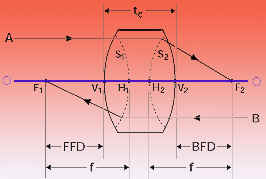 any optical system can be reduced to the specification of the positions of the principal and focal points.

Symbol: Description

O-O1: Optical Axis

F1: Front Focal Point: Common focal point of all rays B parallel to optical axis and travelling from right to left.

V1 Front Vertex: Intersection of the first surface with the optical axis.

S1: First Principal Surface: A surface defined by the intersection of incoming rays B with the corresponding outgoing rays focusing at F1.

H1: First Principal Point: Intersection of the first principal surface with the optical axis.

f Effective Focal Length: The axial distance from the principal points to their respective focal points. This will be the same on both sides of the system provided the system begins and ends in a medium of the same index.

FFD: Front Focal Distance: The distance from the front vertex to the front focal point.

F2 :Back Focal Point: Common focal point of all rays A parallel to optical axis and travelling from left to right.

V2 Back Vertex: Intersection of the last surface with the optical axis.

S2 :Second Principal Surface: A surface defined by the intersection of rays A with the outgoing rays focusing at F2.

H2: Second Principal Point: Intersection of the second principal surface with the optical axis.

BFD: Back Focal Distance: The distance from the back vertex to the back focal point.

Singlet Lenses

Below, we tabulate the focal length, back focal distance, and front focal distance for a general singlet lens and the commonly available singlet lenses plano-convex, plano-concave, bi-convex (actually equiconvex), and bi-concave (actually equiconcave). The sign conventions used are as follows:

a. R is positive when the surface is convex when encountered moving from left to right along the optical axis

b. R is negative when the surface is concave when encountered moving from left to right along the optical axis

c. BFD is positive when F2 is to the right of V2.BFD is negative when F2 is to the left of V2

d. FFD is positive when F1 is to the left of V1

e. FFD is negative when F1 is to the right of V1

f. The first principal point H1 is to the right of F1 for positive f, and to the left of F1 for negative f

g. The second principal point H2 is to the left of F2 for positive f, and to the right of F2 for negative f

Note:the formulas for FFD and BFD depend on the lens orientation when the lens is assymetrical. The formula for f does not depend on orientation. Finally, when R is used without a subscript in the formulas below, it is positive.

Using the formulas below, you can plot out the principal points. Using the formulas for FFD and BFD, find the positions of the front and back focal points with respect to the front and back vertices. Using the value and sign of f, find the first and second principal points.

Spherical Aberration and Spot Size

High quality singlet lenses are of particular interest in laser focusing and beam handling applications because of their low cost, high damage threshold, and the availability of standard parts.

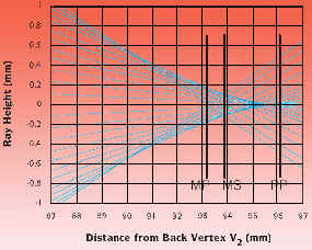
Can singlet lenses provide diffraction limited focusing of collimated beams? Examine the figure above. This figure represents 25 light rays traced near the focal plane of an f =+100mm plano-convex lens of index n = 1.515.

The radius of curvature of the convex surface is R = 51.5mm and its center thickness is tc = 6mm.

The rays start out parallel to the optical axis, and were spaced equally in a region ±16mm above and below it. Therefore the lens is operating at a relatively fast F#

The back focal distance of the lens is:

Clearly, not all rays come to focus in the paraxial focal plane, marked PP in the figure. Only rays very close to the optical axis focus there. Rays that start out farther from the optical axis come to a focus closer to the lens. The marginal rays, which started out 16mm from the optical axis, focus in plane MP. There is a minimum beam diameter dMS which occurs at intermediate plane MS. dMS can be calculated from third order aberration theory. The result is:

where Dq blur is the angular blur of the lens, given by:

d₀ is the initial beam diameter and K is the shape factor of the lens:

The full angular blur is plotted below for singlet lenses as a function of shape factor for various indices of refraction. For n = 1.5, the blur is a minimum for K = 6/7. This describes a bi-convex lens with the flatter side R2 = -6R1. Such a lens is called a best form singlet lens, and will focus to a spot approximately 8% smaller than a plano-convex lens.

In our example of a plano-convex lens of f=+100mm oriented with plano side toward the focus, K = 1. Using d0 = 32mm, we compute dMS = 0.226mm. The wavelength of light has not entered the calculation; this result is a pure geometric optics calculation. The diffraction limited focusing of a uniform 32mm diameter beam by a 100mm lens can be estimated by the diameter of the first minimum of the Airy diffraction pattern in the focal plane. If we take l = 632.8nm, we obtain:

So geometric optics predicts a beam diameter, dMS, due to transverse spherical aberration, which is about 47 times diffraction limited.

In other words, spherical aberration contributes an intrinsic blur, blur, which limits the angular resolution of the lens. At this point Dq(blur)=Dq(diff) we may say that a singlet, if fabricated with high precision, approaches diffraction limited performance.

Singlet or Multiple Elements Lens

Here is a procedure to determine whether a singlet or multiple element lens will be needed to achieve the required spot size.

1. Determine the spot size dspot needed for the experiment.
2. Calculate the required focal length from the divergence properties of the beam.

For a TEM00 gaussian beam, use:

where w0 and wspot are the initial and desired beam waists. This formula is an excellent approximation when the distance from the initial waist w0 to the front focal plane is much smaller than the initial confocal parameter z0 =w02 /.

For a plane wave truncated by an aperture d0 use:

For a non-diffraction limited laser beam, use:

where full is the measured or manufacturer specified full angle divergence.

3. Calculate the blurred focal spot due to spherical abberation, using the shape factor, index of refraction, and initial beam diameter:

For a properly oriented plano-convex lens of index n = 1.5, the bracketed factor is 0.073.

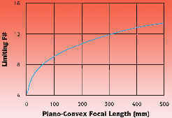
If the blurred focal spot size is greater than or equal to the desired spot size, a multi-element lens is required to achieve the desired spot size. This lens selection rule is based on blur as a result of spherical aberration compared with blur due to diffraction. It can be formulated as a limiting f#. For plane wave focusing:

Using

we obtain the condition

To achieve diffraction limited focusing, the f# has to be greater, or the speed of the single element lens "slower" than this expression containing the focal length. As an example, see the graph below.

Polarization States

Four numbers are required to describe a single plane wave Fourier component traveling in the +z direction. These can be thought of as the amplitude and phase shift of the field along two orthogonal directions.

a. Cartesian Representation

This is the simplest representation to think about. Ex , Ey, fx, and fy are four real numbers describing the magnitudes and phases of field components along two orthogonal unit vectors x and y. If the origin of time is irrelevant, only the relative phase shift need be specified.

b. Circular Representation

In the circular representation, we resolve the field into circularly polarized components. The basic states are represented by the complex unit vectors:

e+ is the unit vector for left circularly polarized light; for positive helicity light; for light that rotates counterclockwise in a fixed plane as viewed facing into the light wave; and for light whose electric field rotation obeys the right hand rule with thumb pointing in the direction of propagation.

e-is the unit vector for right circularly polarized light; for negative helicity light; for light that rotates clockwise in a fixed plane as viewed facing into the light wave; and for light whose electric field rotation disobeys the right hand rule with thumb pointing in the direction of propagation.

As in the case of the Cartesian representation, we write:

where E+ , E-, +, and - are four real numbers describing the magnitudes and phases of the field components of the left and right circularly polarized components. Note that:

c. Elliptical Representation

An arbitrary polarization state is generally elliptically polarized. This means that the tip of the electric field vector will describe an ellipse, rotating once per optical cycle.

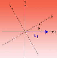
Let a be the semimajor and b be the semiminor axis of the polarization ellipse. Let be the angle that the semimajor axis makes with the X-axis. Let and be the axes of a right-handed coordinate system rotated by an angle + with respect to the X-axis and aligned with the polarization ellipse as shown in the diagram below.

The elliptical representation is:

Note that the phase shift o above is required to adjust the time origin, and the parameter is implicit in the rotation of the , axes with respect to the X, Y axes.

Conversion Between Representations

For brevity, we will provide only the Cartesian to Circular and Cartesian to Elliptical transformations. The inverse transformations are straightforward. We define the following quantities:

In the above, atan(x,y) is the four quadrant arc tangent function. This means that atan(x,y) = atan(y/x) with the provision that the quadrant of the angle returned by the function is controlled by the signs of both x and y, not just the sign of their quotient. For example, if g₂ = g₁ = -1, thenφ₁₂ above is 5π/4 or -3π/4, notπ/4.

a. Cartesian to Circular Transformation

b. Cartesian to Elliptical Transformation

Linear Polarizers

A linear polarizer is a device that creates a linear polarization state from an arbitrary input. It does this by removing the component orthogonal to the selected state. Some polarizers reflect the rejected state, creating a new, usable beam. Others may turn the rejected beam into heat, as do polaroid sheet and PolarcorTM polarizers.

Still others may refract the two polarized beams at different angles, thereby separating them. Examples are Wollaston and Rochon prism polarizers.

Suppose the pass direction of the polarizer is determined by unit vector p. Then the transmitted field E2, in terms of the incident field E1, is:

where the phase shift of the transmitted field has been ignored.A real polarizer has a pass transmission, T||, less than 1. The transmission of the rejected beam, T, may not be 0. If r is a unit vector along the rejected direction, then

In the above, the phase shifts along the two directions must be retained. Similar expressions could be arrived at for the rejected beam. If q is the angle between the field E1 and the polarizer pass direction p, the above equation predicts for the transmission:

The above equation shows that when the polarizer is aligned so that θ= 0, T = T_||. When it is "crossed",θ=π/2, and T = T┴. The extinction ratio is ε= T_|| /T┴.

A polarizer with perfect extinction has T┴= 0, and thus T = T|| cos²θ, is a familiar result. Because cos2 has a broad maximum as a function of orientation angle, setting a polarizer at a maximum of transmission is generally not very accurate. One has to either map the cos²θ with sufficient accuracy to find the θ= 0 point, or do a null measurement at θ= π± /2.

Waveplates

Waveplates operate by imparting unequal phase shifts to orthogonally polarized field components of an incident wave. This causes the conversion of one polarization state into another.

There are two cases. With linear birefringence, the index of refraction and hence phase shift differs for two orthogonally polarized linear polarization states. This is the operation mode of standard waveplates.

With circular birefringence, the index of refraction and hence phase shift differs for left and right circularly polarized components. This is the operation mode of polarization rotators.

a. Standard Waveplates: Linear Birefringence

Suppose a waveplate made from a uniaxial material has light propagating perpendicular to the optic axis. This makes the field component parallel to the optic axis an extraordinary wave and the component perpendicular to the optic axis an ordinary wave. If the crystal is positive uniaxial, ne > no, then the optic axis is called the slow axis, which is the case for crystal quartz. For negative uniaxial crystals, ne < no, the optic axis is called the fast axis.

The equation for the transmitted field E2, in terms of the incident field E₁ is:

where s and f are unit vectors along the slow and fast axes. This equation shows explicity how the waveplate acts on the field. Reading from left to right, the waveplate takes the component of the input field along its slow axis and appends the slow axis phase shift to it. It does a similar operation to the fast component.

The slow and fast axis phase shifts are given by:

where ns and nf are, respectively, the indices of refraction along the slow and fast axes, and t is the thickness of the waveplate.

To further analyze the effect of a waveplate, we throw away a phase factor lost in measuring intensity, and assign the entire phase delay to the slow axis:

I the above, Δn(λ) is the birefringence n_s(λ) - n_f(λ). The dispersion of the birefringence is very important in waveplate design; a quarter waveplate at a given wavelength is never exactly a half waveplate at half that wavelength.

Let E1 be initially polarized along X, and let the waveplate slow axis make an angle ξ with the X-axis. This orientation is shown in the figure below.

When the waveplate is placed between parallel and perpendicular polarizers the transmissions are given by:

Note: is only a function of the waveplate orientation, and f is only a function of the wavelength, the birefringence is a function of wavelength and the plate thickness.

For a full waveplate:
φ = 2mπ, T_|| = 1, and T┴= 0, regardless of waveplate orientation.

For a half waveplate:
φ= (2mπ + 1), T_|| = cos₂2θ, and ┴T= sin₂2θ.

This transmission result is the same as if an initial linearly polarized wave were rotated through an angle 2θ. Thus, a half waveplate finds use as a polarization rotator.

For a quarter waveplate:
φ= (2mπ + 1)/2; i.e. an odd multiple of π/2. To analyze this, we have to go back to the field equation. Assume that the slow and fast axis unit vectors s and f form a right-handed coordinate system such that s x f = +z, the direction of propagation. To obtain circularly polarized light, linearly polarized light must be aligned midway between the slow and fast axes. There are four possibilities listed in the table below.

b. Multiple Order Waveplates

For the full, half, and quarter waveplate examples given in the preceeding section, the order of the waveplate is given by the integer m. For m > 0, the waveplate is termed a multiple order waveplate. For m = 0, we have a zero order waveplate.

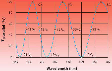
The birefringence of crystal quartz near 500nm is approximately 0.00925. Consider a 0.5mm thick crystal quartz waveplate. A simple calculation shows that this is useful as a quarter waveplate for 500nm; in fact, it is a 37/4 waveplate at 500nm with m = 18. Multiple order waveplates are inexpensive, high damage threshold retarders. Further analysis shows that this same 0.5mm plate is a 19l/2 half waveplate at 488.2nm and a 10 full waveplate at 466.5nm. The transmission of this plate between parallel polarizers is shown in the above figure as a function of wavelength. The retardance of the plate at various key points is shown. Note how quickly the retardance changes with wavelength. Because of this, multiple order waveplates are generally useful only at their design wavelength.

c. Zero Order Waveplates

As discussed above, multiple order waveplates are not useful with tunable or broad bandwidth sources (example: femtosecond lasers). A zero order waveplate can greatly improve the useful bandwidth in a compact, high damage threshold device.

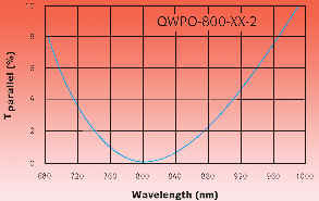
As an example, consider the design of a broadband half waveplate centered at 800nm. Maximum tuning range is obtained if the plate has a single p phase shift at 800nm. If made from a single plate of crystal quartz, the waveplate would be about 45mm thick, which is too thin for easy fabrication and handling. The solution is to take two crystal quartz plates differing in thickness by 45 mm and align them with the slow axis of one against the fast axis of the other. The net phase shift of this zero order waveplate is . The two plates may be either air-spaced or optically contacted. The transmission of an 800nm zero order half waveplate between parallel polarizers is shown in the figure below using a 0-10% scale. Its extinction is better than 100:1 over a bandwidth of about 95 nm centered at 800nm.

d. Achromatic Waveplate

At 500 nm, a crystal quartz zero order half waveplate has a retardation tolerance of l/50 over a bandwidth of about 50nm. This increases to about 100nm at a center wavelength of 800nm. However, there is a waveplate design that can give an even larger bandwidth.

If two different materials are used to create a zero or low order waveplate, cancellation can occur between the dispersions of the two materials. This requires a judicious choice of thicknesses. Then, the net birefringent phase shift can be held constant over a much wider range than in waveplates made from one material. The ACWP-series crystal quartz and MgF2 Achromatic Waveplates are used in high power, air-spaced designs.

Three wavelength ranges are available in both quarter and half wave retardances. Retardation tolerance is better than /100 over the entire wavelength range. We plot the intensity transmission and the actual phase shift for each design versus wavelength. For quarter waveplates, perfect retardance is a multiple of 0.25 waves, and transmission through a linear polarizer must be between 33% and 67%. (In all but the shortest wavelength design, quarter wave retardation tolerance is better than /100.) For half waveplates, perfect retardance is 0.5 waves, while perfect transmission through a linear polarizer parallel to the intitial polarization state should be zero.

e. Dual Wavelength Waveplates

Dual wavelength waveplates have a number of applications. One common appliction is separation of different wavelengths with a polarization beam splitter by rotating the polarization of one wavelength by 90°, and leaving the other unchanged. This application frequently occurs in nonlinear doubling or tripling laser sources such as Nd:YAG (1064/532/355/266).

In single waveplate applications, a more robust approach is to combine two quartz waveplates with their optical axes orthogonal to one another. In this configuration, the temperature dependence is a function of the thickness difference between the waveplates, resulting in excellent temperature stability. The retardation of the compound waveplate is also a function of the thickness difference, so a zero order waveplate can be realized, resulting in a very wide bandwidth.

f. Low Order Dual Wavelength Waveplates

Low order dual wavelength waveplates offer the temperature and stability of a zero order waveplate while still meeting the specified retardation at two different wavelengths. These high energy air- spaced waveplates, made of magnesium flouride and crystal quartz, are perfect for OPOs, spectrophotometry, femtosecond pulses, and continuum generation. In addition, low order dual waveplates can rotate the polarization of a single wavelength while not affecting the polarization of a second wavelength.